
Making Good Measurements for Automated Test
There are many causes of test inaccuracies. Understanding that equipment measurement accuracy, repeatability, unit capabilities, test limits, and the specification, is the first step to limiting the effect of testing variances on UUT pass/fail errors. This understanding provides large cost and labor savings in the production, test, and product acceptance phases.
When bad product is found in the field, potentially huge costs can be incurred:
- as warranty claims,
- as service calls,
- or as disgruntled customers upset by a requirement failure.
No one wants to ship bad product. But did you know that even if you have a calibrated device (i.e., sensor, instrument, or test station), you can still pass a bad product? Your immediate question might be “How can a test pass but the unit fail?”.
Other Motivators
- Perhaps, you have had vendors provide you parts that they claimed were tested only to have your incoming inspection reject the parts because they don’t pass?
- Or possibly the reverse has happened to you where you have shipped parts to a customer and the customer claims they don’t pass.
Hopefully, these cases are few and far between because when they happen they typically require extensive time, questioning, and possibly re-validating the test method. The cause of this potentially costly effort is typically based on a misunderstanding of the test system accuracy.
Even though you are diligent about the calibration of your test equipment or test system, it is still possible that your test has allowed a product to be passed despite having actually failed. This situation is called a false positive. The reason false positives occur is explained below.
Common Scenarios
It’s important to understand that all test equipment has accuracy specs. Typically, these specs are listed among the other specifications and generally ignored because they are misunderstood and small relative to normal readings. But, measurement accuracy can be the cause of passing a failing unit if the performance of the unit under test (UUT) is close to a product specification limit.
Typically, engineers or test authors try to manage the testing by keeping the limits centered on the usual product performance. Due to typical product variations, sometimes the product performance is close to a limit. If the product performance variations are skewed or shifted towards one of the limits, your product will approach the limit more frequently. When the UUT performance is close to a limit, the measurement equipment accuracy can allow a failing unit to have measurement readings appear that it passed. A false positive has occurred.
Here are some descriptions, based on actual scenarios, which help describe this condition:
- You pass the UUT when the rise time measures 99 ns, which is within 1 ns of the 100 ns high limit specification, but the measurement device has a tolerance of ±5 ns. Should the UUT be passed?
- Your spectrum analyzer stops functioning, and the replacement analyzer fails more UUTs for measured spectral amplitudes or frequencies that are higher than before. Both analyzers are calibrated, so why is there an issue?
- Your scope needs calibrating, and the only replacement scope has a lower bandwidth but this was not recognized until parts start failing more than usual. They were both calibrated, so what’s going on?
- Your customer is using a measurement device to validate compliance at incoming inspection or field test. The device is less accurate than the one used in production to test the unit. The product passed at the product test system but, because of the inaccuracy of the customer’s inspection equipment, it looks to the customer that you have provided non-compliant product. Are you prepared for the ensuing discussion?
Definitions
There are many terms that are used to describe measurement system variations. Here’s a list to get you started (these issues are often discussed under the topic of Measurement System Analysis (MSA)).
- Accuracy: A measure of how close a measured value is to the “true” value.
- Precision: The variability of a measurement.
- Tolerance: The manufacturer’s stated uncertainty in the accuracy of a device. This value is typically listed to alert the user of the inaccuracies of the equipment.
- Repeatability: The variation in measurements taken by a single person or instrument on the same item and under the same conditions.
- Reproducibility: The variability induced by the operators. It is the variation induced when different operators (or different laboratories) measure the same part.
These terms all relate to the statistical variations that occur in a measurement system. Usually, these terms relate to ±3 standard deviations but sometimes they are reported as ±1 or ±2, so beware. Also, I’ve never seen a good statistical definition of tolerance but I think of it as including variations due to drift in accuracy and short term noise from precision variations.
Accuracy and Precision
The two bulls-eye diagrams below illustrate the difference between accuracy and precision. The accurate source has the average value centered on the bulls-eye.

Accurate source
Many people confuse the other bulls-eye as being more accurate since the points are clustered more tightly.

Precise source
The points in the second figure are more precise, but, since they do not surround the bulls-eye, they are not accurate. A device with stable output is a precise device. Stability does not imply a correct value. In technical terms, the accurate source figure has a larger standard deviation (SD) than the precise source, but a correct mean value.
False Positives and Negatives
The equipment measuring a UUT has a known accuracy and precision based on the results of the equipment calibration. Equipment with multiple measurement ranges typically has different accuracy and precision for each range as a percent of range. These variations combine to make any specific measurement uncertain. Look at the situation where the measurement equipment measures a value close to a UUT pass/fail limit. Sometimes, due to variations in the measurement equipment, the UUT performance appears to fall outside the limits, even though the UUT actually performed within the limits. In other words, the UUT will fail the test, even though it should have passed, resulting in a false negative. The opposite can also happen when the UUT is measured as being within the limits even though the actual performance is outside the limits, resulting in a false positive. These incorrect determinations are caused by the equipment measurement variations or inaccuracy and are called Type 1 (false negative) and Type 2 (false positive) errors, respectively, in the statistics world. Figure 1 below shows the issue.
Figure 1. Measurements and part variations
Figure 1 shows the measurement variation at the low and high test limit locations but measurement variation occurs everywhere and becomes especially interesting and important at the edges.
Recall Scenario 1 above, where the high test limit in Figure 1 is 100 ns for a pulse rise time. The equipment, which has an accuracy of ±5 ns, measures 99 ns. Does the test pass or fail? A measurement of 99 ns with an accuracy of ±5 ns means the actual reading is really anywhere between 94 ns and 104 ns. Typically, the test engineer might think that using a bell curve (also known as a normal or Gaussian distribution) is reasonable and that the reading is “probably” 99 ns but, as Figure 1 illustrates, the actual value could be higher or lower.
To make matters more complicated, equipment vendors are not required to provide readings with variations that follow a bell curve. In fact, variations may not be equally distributed. Some equipment may be biased in one direction and other equipment may properly trend to the nominal reading value. If your measurement is close to the test limit and especially if readings are biased low, then it is possible that the equipment reads 99 ns when the unit is actually producing, say, 102 ns.
One method to handle this pass/fail uncertainty is to stay away from these limits by using “guard bands” within the limit range. These guard bands would be proportional in width to deviations in measurements caused by accuracy and precision tolerances.
So, in Scenario 1 above, you should not pass the UUT when the rise time is within 1 ns of the specification limit but the measurement device has a calibrated accuracy of ±5 ns. In this case, a specification limit of 100 ns would need equipment measurements of 95 ns or less for the test to prove conclusively that the unit passed. Note, “conclusively” means 99.7% certainty when the ±5 ns equals ±3 standard deviations (SDs) of the equipment variations. Other SDs will give different certainties.
Figure 2 shows the same product test limits with the measurement accuracy accounted by providing production test limits. The production test limits illustrate that guard bands reduce the measurement error that falls outside the product limits. Note, however, that using guard bands bring up an additional issue because now you are constraining the design to meet a 95 ns limit so that your design can meet your specification. This situation may not be desirable or possible if your unit naturally exhibits behavior close to the test limits.
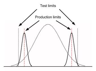
Figure 2 – Production limits using guard bands to reduce false positives
The popular Six Sigma approach tries to reduce variations in the product so that the part variations become narrower. Thus, without moving the test limits or adding guard limits, there are less (hopefully many less) Type 2 (and Type 1) errors. This concept is illustrated in Figure 3 which shows a narrowed part variation bell curve. We’ve also included an offset (also called bias) shifting the center of the part variations towards the upper limit, as can happen in actual production.
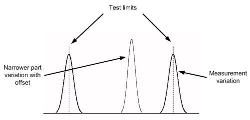
Figure 3 – Six Sigma reduces part variations
In general, you should be considering that there are 4 types of measurement outcomes, as indicated in the 2×2 chart in Figure 4 from Reference 2.
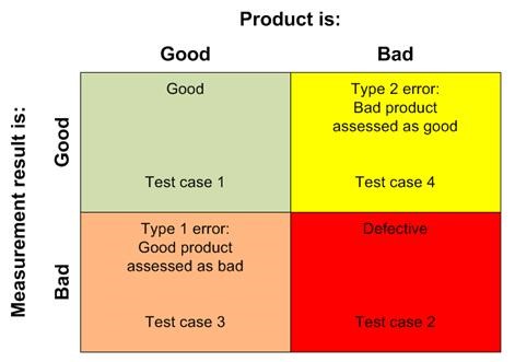
Figure 4 – Various actual pass/fail outcomes and their causes
Generally, only test cases 1 and 2 are considered. Nevertheless, outcomes indicated by the other test cases are possible. We’ve been discussing the Type 2 errors in the upper right of this chart. The goal of any test system is to reduce these Type 2 errors. The test case 3 is also of interest since it causes internal diagnostic and rework when none is needed and the associated costs could be avoided.
Equipment Accuracy
In Scenarios 2 and 3, since the measured values from the replacement equipment tend to fail more parts than the original equipment, assuming they are both calibrated, the accuracy of the replacement equipment must be worse than the replaced equipment. The measurement variations around the limits shown in Figure 1 are wider and more often fall outside the upper limit. There are more Type 1 errors.
Accuracy may be affected by environmental conditions and internal noise-generating processes. Environmental conditions tend to cause long term drift. If you think about the bulls-eye diagram, the accuracy might show measurement variations out to the 4th ring diameter, but over any short duration in time, the precision of the instrument might gather repeated measurements into a tight cluster that wanders around inside the 4th ring. This clustering fools the operator into thinking the readings are super accurate when they are not. Thus, the equipment in Scenarios 2 and 3 can provide a consistently higher reading because it has drifted away from the center of the bulls-eye despite being within the accuracy spec.
Equipment Capability
Equipment that has been replaced by more modern digital measurement equipment often has improved performance and statistical processing capabilities. Beyond increased precision (i.e., more digits on the readout), you might also see better accuracy (less variance), wider bandwidth, and so on. I have seen many cases where the product engineers are scratching their heads wondering why their product is not passing operating specifications when the new equipment now measures behaviors they never knew existed.
We once delivered an upgraded test system that was so responsive and precise that all parts failed an in-rush test: the original test equipment did not respond to the initial current pulse.
This scenario occurs because many test specifications are written based on typical behavior of part performance measured with a certain piece of equipment, e.g., the one the design engineer used in the lab. Unfortunately, sometimes production, incoming inspection, or field service does not have the budget for the “expensive” test equipment that design engineering gets to use, so they use less expensive equipment and may introduce errors as a result. These errors are exhibited in the above Scenarios 3 and 4.
Next Steps
The ultimate goal of this effort is to make sure that no product leaves the factory that is a Type 2 error (bad product passing as good) and production is not trying to troubleshoot a Type 1 error (good product indicated as failed). These types of errors are extremely costly and even worse if found in the field, as a warranty claim, or by the customer, as a requirement failure or non-compliance. Therefore, close attention must be paid to maintaining a consistent testing configuration and fully understanding the test and measurement accuracy, precision, and repeatability of the equipment that make up the test environment.
Want some help with your test system?
Deep into learning mode? Check these out:
- Commissioning Custom Test Equipment
- 9 Considerations Before you Outsource your Custom Test Equipment Development
- Test Automation Best Practices – for automated hardware testing
- Product Testing Methods – for industrial hardware products
- Universal Test Equipment – An Argument against it
- 5 Keys to Upgrading Obsolete Manufacturing Test Systems
- Hardware Test Plan – for complex or mission-critical products
References
- https://benthamopen.com/ABSTRACT/TOIMEJ-1-29
- Background on Type 1 and 2 errors: https://en.wikipedia.org/wiki/Type_I_and_type_II_errors.